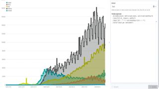
How to visualize complex data on Linux
Simon Quain shows how to visualize Covid-19 statistics and more with freely available open datasets and Timelion, a plugin for Elasticsearch.
Making use of offsets
Sometimes you want to be able to see how your data compares to the previous week, day or year. Whether that’s the number of sales this week compared to last week or year, or the count of http error responses in your logs compared to yesterday. Timelion has the offset function that enables us to do just this.
Let’s write a Timelion expression to compare the number of cases in England compared to the number of cases in Italy two weeks previously:
.es(index=covid, q="countriesAndTerritories: United_Kingdom”, metric=sum:cases).label("UK Cases"),
.es(index=covid, q="countriesAndTerritories: Italy”, metric=sum:cases, offset="-2w").label("Italian Cases two weeks ago")

How about showing how much the number of cases has increased or decreased compared to the previous week in the United Kingdom?
We can do this with the subtract() function:
.es(index=covid, q="countriesAndTerritories: United_Kingdom”, metric=sum:cases).label("UK Cases"),
Are you a pro? Subscribe to our newsletter
Sign up to the TechRadar Pro newsletter to get all the top news, opinion, features and guidance your business needs to succeed!
.es(index=covid, q="countriesAndTerritories: United_Kingdom”, metric=sum:cases).subtract(
.es(index=covid, q="countriesAndTerritories: United_Kingdom”, metric=sum:cases, offset=-1w)).bars().
label("UK Cases vs Previous Week")
Note how you can put entire Timelion expressions within other Timelion functions. There are also multiply and divide functions, among others.
This is not normal
We can take our work with moving averages further with the .holt() function. It’s used to compare what should be happening right now to what’s actually happening.
Instead of having past observations weighted equally, you can control how important certain variables are in determining the current value. The three variables that the .holt() function takes are alpha, beta and gamma and they all take values between 0 and 1.
Alpha is a weighted moving average that determines how important the days immediately preceding are. The higher this number is, the less important they are. Beta is for the trend and determines how much weight you give to the fact that the trend is going up or down.
For this, small values emphasise long-term trends, while larger values are for short-term trends. Gamma is the seasonality of the data. Seasonality deals with regular and predictable patterns in your data such as traffic patterns on a busy road or to your website over a week.
Here we can adjust how much weight last Tuesday’s data should have on determining what this Tuesday’s data should look like. If you’re using seasonality you can add a further parameter that tells Timelion what the seasonality is. For weekly you would put “1w”.
Creating a graph with the .holt() function will be a matter of adjustment depending on your data. The Covid data we have doesn’t have a seasonality trend, so here’s an example using the alpha and beta values to compare what it thinks should be happening against what’s actually happening.
.es(index=covid , metric=sum:cases).holt(0.5, 0.2).label("Holt"),
.es(index=covid , metric=sum:cases).label("Cases")
You can spend some time tweaking these values to see how the graphs change in front of you and where the observed value deviates from the predicted value.
Timelion often doesn’t get the attention it rightly deserves. We hope we’ve shown you how much you can do with this versatile visualisation tool and freely available open datasets. Of course, there hasn’t been space to cover all that it can do in these five pages.
As next steps you could have a look at the .if() function to use conditionals in your expressions, fill in gaps in your data with the fill() function, plot the rate of change with .derivative() and go further with the Mathlion extension, which enables equation parsing and advanced maths in Timelion.
